3-Machine Learning

elementsofai.com

Published

February 26, 2025

Note

When fundraising: it’s AI
When recruiting: it’s machine learning
When implementing: it’s linear regression

AI is a broad and often exciting term that encompasses many different technologies. When recruiting, you’ll need to be more specific and talk about areas like machine learning. When implementing AI solutions, discussions become even more focused on specific methods, such as linear regression, neural networks, or decision trees, depending on the problem at hand.

Supervised learning

We know what the answer is and we try to build a model to generate correct answers.

Example: You have data about prices and surface of appartments and you train an AI to predict appartment prices. Or, you train an AI to identify animals in pictures.

Linear Regression

This is a method of predicting results based in a function.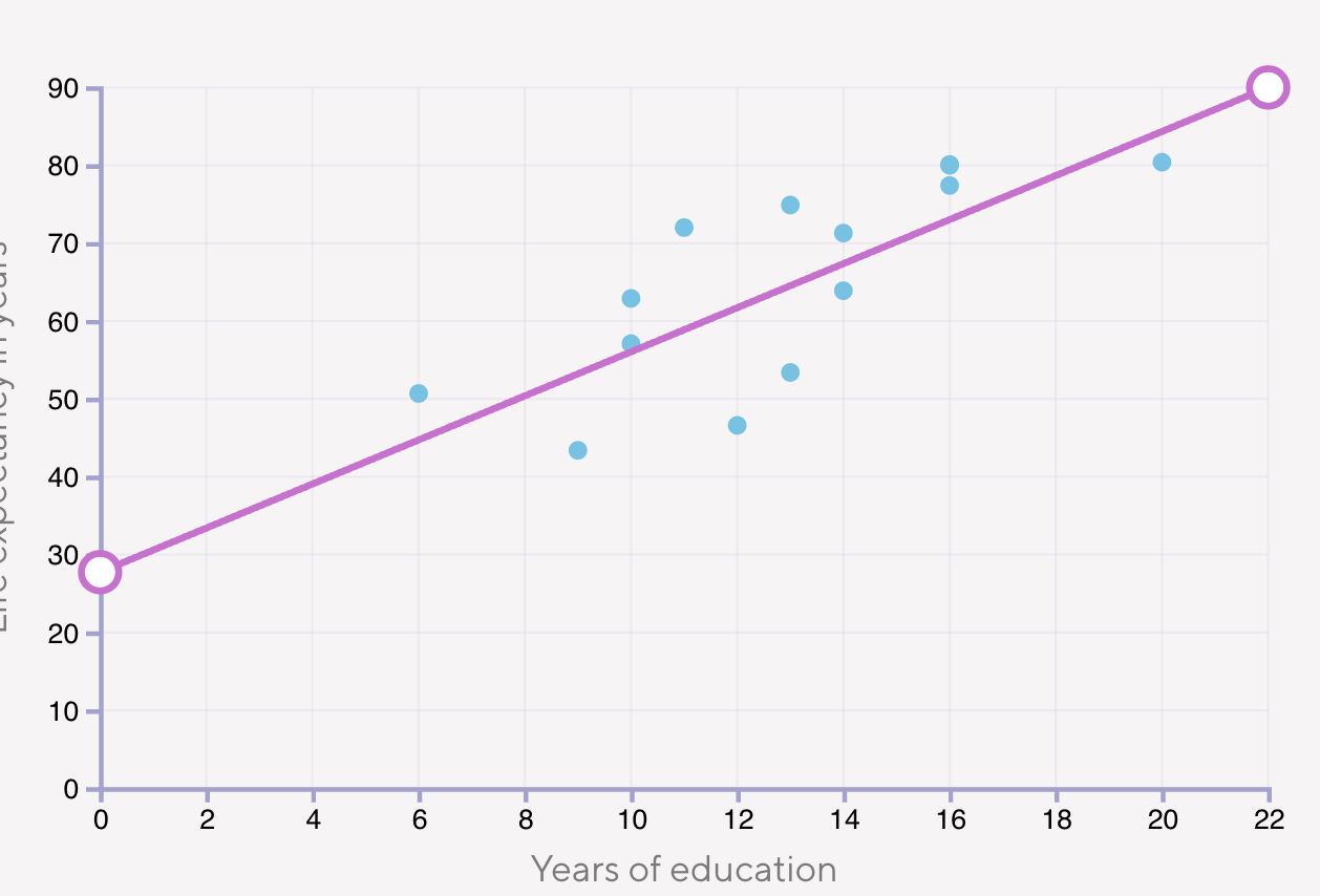

with this function we can predict that someone who lives in a country where the average year of education is 15 has a life expectancy probably between 50 an 90 year.

Simple Linear Regression

One independent variable (x) predicting one dependent variable (y).
Needs at least two points to define a line.
Equation: \(y=mx+b\)
Example: Predicting height based on age.

Multiple Linear Regression

Two or more independent variables (\(x_1\), \(x_2\), \(x_3\), …) predicting one dependent variable (y).
Equation: \(y = w_1 x_1 + w_2 x_2 + ... + w_n x_n + b\)
Example: Predicting house price based on size, number of bedrooms, and location.

We’ll mostly work with prices for holiday cabbins (called mökkis in Finland) and their price corresponding to multiple selling arguments.

In linear regression the price of cabin would change depending of how far it is from a body of water, but it will also change depending on the size or how many toilets it has. To take into account these multiple variables to reach a prediction, we would need to do some tricks: for example, predict the price per square meter of a cabin depending on how close it is to a body of water and then use it to calculate the final price.

For multiple parameters where we trained an AI (=calculated the estimated coefficients) we would then predict the price like this:

# input values for one mökki: size, size of sauna, distance to water, number of indoor bathrooms, 
# proximity of neighbours

x = [66, 5, 15, 2, 500]
c = [3000, 200 , -50, 5000, 100]     # coefficient values

prediction = c[0]*x[0] + c[1]*x[1] + c[2]*x[2] + c[3]*x[3] + c[4]*x[4]

*For a mökki of 66\(m^2\), 5\(m^2\) of sauna, 15\(m\) from the water, 2 bathrooms and 500\(m\) to the nearest neighbour the predicted price would be 258250€

Or calculate the price prediction of multiple cabins with:

# input values for three mökkis: size, size of sauna, distance to water, number of indoor bathrooms, 
# proximity of neighbors
X = [[66, 5, 15, 2, 500], 
     [21, 3, 50, 1, 100], 
     [120, 15, 5, 2, 1200]]
c = [3000, 200, -50, 5000, 100]    # coefficient values

def predict(X, c):
    for i,x in enumerate(X):
        price = sum(c[i] * x[i] for i in range(len(c)))
        ordinal="st" if i==0 else "nd" if i==1 else "rd"
        print(f"{str(i+1)}{ordinal} mökki is predicted to cost {str(price)}€")

predict(X, c)

1st mökki is predicted to cost 258250€
2nd mökki is predicted to cost 76100€
3rd mökki is predicted to cost 492750€

see that we used sum(…) to add all the parameters in a loop which, imagine that there are 50 parameters, it would be cumbersome to write them all

A libary can also do these calculations easily without explicitly writing loops:

import numpy as np

x = np.array([66, 5, 15, 2, 500])
c = np.array([3000, 200 , -50, 5000, 100])
one_predictions=x @ c

x = np.array([[66, 5, 15, 2, 500], 
              [21, 3, 50, 1, 100]])
two_predictions=x @ c

with 1 dimentional array as input : 258250
with 2 dimentional array as input : array([258250, 76100])

Now all of this is not artificial intelligence is it?

Least squares formula

We can instead of predicting the prices, estimate the coefficients to then predict the prices. For that, we’ll need the price and data of multiple mökkis that will be used to “train” the AI.

Estimating the parameters in linear regression is one of the classical problems in statistics and machine learning, and the most classical solution to this classical problem is the so-called least squares method proposed by Legendre and Gauss in the beginning of the 1800.

Optional - learn the calculations in deapth

To explain this method lets imagine the following table of time spent studying and score in a test! There are python packages doing this for us and these calculations are purely for understanding the method

time	score
1	60%
2	65%
3	70%
4	75%
5	85%

We’re looking for the y = mx + b that minimizes the sum of squared errors:

1. calculate the means of x and y:

\(x̄ = (1 + 2 + 3 + 4 + 5) / 5 = 15 / 5 = 3\)
\(ȳ = (60 + 65 + 70 + 75 + 85) / 5 = 355 / 5 = 71\)

2. Step 2: Calculate the slope (m) using the formula:

\(m = Σ[(x_i - x̄)(y_i - ȳ)] / Σ[(x_i - x̄)²]\)

x	y	x-x̄	y-ȳ	(x-x̄)(y-ȳ)	(x-x̄)²
1	60	-2	-11	22	4
2	65	-1	-6	6	1
3	70	0	-1	0	0
4	75	1	4	4	1
5	85	2	14	28	4

\(Σ[(x_i - x̄)(y_i - ȳ)] = 22+6+0+4+28 = 60\)

\(Σ[(x_i - x̄)²] = 4+1+0+1+4 = 10\)

\(m = 60/10 = 6\)

3. calculate the b using the formula:

\(b = ȳ - m·x̄ = 71 - 6·3 = 71 - 18 = 53\)

so our function would be \(y = 6x + 53\)

4. verify by calculating the predicted values and errors

x	actual y	predicted y	error	squared error
1	60	6(1) + 53 = 59	1	1
2	65	6(2) + 53 = 65	0	0
3	70	6(3) + 53 = 71	-1	1
4	75	6(4) + 53 = 77	-2	4
5	85	6(5) + 53 = 83	2	4

This formula porvides the optimal linear solution

Use python packages for more complex problems

To start with, let’s find the best coefficients from a list of 3 different porpositions. We can calculate the predictions, compare them with the actual values and get the sum of the squared errors to find which sum is the smallest:

import numpy as np

# data
X = np.array([[66, 5, 15, 2, 500], 
              [21, 3, 50, 1, 100], 
              [120, 15, 5, 2, 1200]])
y = np.array([250000, 60000, 525000])

# alternative sets of coefficient values
c = np.array([[3000, 200 , -50, 5000, 100], 
              [2000, -250, -100, 150, 250], 
              [3000, -100, -150, 0, 150]])   

def find_best(X, y, c):
    smallest_error = np.Inf
    best_index = -1
    for i, coeff in enumerate(c):
        # Calculate predictions for this coefficient set
        predictions = np.dot(X, coeff)
        
        # Calculate squared errors
        errors = y - predictions
        squared_errors = errors ** 2
        sse = np.sum(squared_errors)
        
        # Check if this is better than the current best
        if sse < smallest_error:
            smallest_error = sse
            best_index = i
            
    print("the best set is set %d" % best_index)


find_best(X, y, c)

the best set is set 1

And to calculate the coefficients we have numpy.linalg.lstsq

import numpy as np


x = np.array([
             [25, 2, 50, 1, 500], 
             [39, 3, 10, 1, 1000], 
             [13, 2, 13, 1, 1000], 
             [82, 5, 20, 2, 120], 
             [130, 6, 10, 2, 600]
            ])   
y = np.array([127900, 222100, 143750, 268000, 460700])

c = np.linalg.lstsq(x, y, rcond=None)[0]
y_pred = x @ c

print(f"predicted coefficents are {c}")
print("predictions are : \t\t" + str('\t'.join(map(str, y_pred))))
print("actual values are : \t" + str('\t\t\t\t'.join(map(str, y))))

predicted coefficents are [3000.  200.  -50. 5000.  100.]
predictions are :       127900.00000000009  222100.00000000006  143750.00000000003  268000.0000000002   460700.0000000002
actual values are :     127900              222100              143750              268000              460700

the model is always able to perfectly match the output values used as the data if the number of cases is less than or equal to the number of coefficients in the model. In the above example, both are five so the perfect match is actually no surprise after all.

Predictions with more data

Now let’s do predictions with data from a csv file.

Also let’s see the difference when we add a intercept.

The intercept is the b in ax+b, without the intercept we are forcing the function to go through 0,0 which is not true in most cases

To add the intercept we add a column to the entry values with a 1

def fit_model(input_file):
    data = np.genfromtxt(input_file, delimiter=',', skip_header=1)
    
    x = data[:, :-1]
    y = data[:, -1]

    c = np.linalg.lstsq(x, y, rcond=None)[0]
    y_pred = x @ c

    print("predicted coefficents are " +str('\t'.join(map(str, c))))
    print()
    print("predictions are : \t\t" + str('\t'.join(map(str, y_pred))))
    print("actual values are : \t" + str('\t\t\t'.join(map(str, y))))

def fit_model_alt(input_file):
    data = np.genfromtxt(input_file, delimiter=',', skip_header=1)
    
    X = data[:, :-1]
    y = data[:, -1]

    # Add intercept term
    X_with_intercept = np.column_stack([np.ones(X.shape[0]), X])
    c = np.linalg.lstsq(X_with_intercept, y, rcond=None)[0]
    y_pred=X_with_intercept @ c

    print("predicted coefficents are " +str('\t'.join(map(str, c))))
    print()
    print("predictions are : \t\t" + str('\t'.join(map(str, y_pred))))
    print("actual values are : \t" + str('\t\t\t'.join(map(str, y))))

fit_model('../../resources/data/mokki.csv')
print("\n------------------\nNow with intercept\n------------------\n")
fit_model_alt('../../resources/data/mokki.csv')

predicted coefficents are 2989.626782447968 800.6106446281458   -44.79961627495003  3890.7925855158737  99.82970234993199

predictions are :       127907.55379718984  222269.77522205355  143604.46938495338  268017.6065113987   460686.5560042461   406959.8765645142
actual values are :     127900.0            222100.0            143750.0            268000.0            460700.0            407000.0

------------------
Now with intercept
------------------

predicted coefficents are 12530.995817391788    3082.486428762153   -2235.4898994402024 -146.947583874725   2722.4259143895683  94.80555308356193

predictions are :       127899.99999999948  222099.9999999994   143749.99999999945  267999.99999999936  460699.99999999953  406999.99999999953
actual values are :     127900.0            222100.0            143750.0            268000.0            460700.0            407000.0

Nearest neighbor

Linear regression is a definite classic among the countless machine learning methods borrowed from statistics. Among the more recent methods that have been invented by computer scientists the so-called nearest neighbor method is an equally classic technique.

The nearest neighbor method can be used for both regression and classification tasks (like vector databases for example). For it we need to have a formula to calculate distance. In a map for example (2d pane) we can use the pythagorean theory to calculate the distance between Lisbon and Geneva.

\(D_{\text{LIS, GVA}}=\sqrt{(X_{\text{LIS}}-X_{\text{GVA}})^2 + (Y_{\text{LIS}}-Y_{\text{GVA}})^2}\)

In this same way, we can calculate the difference (or distance) of a mökki with 34m2 and 10m from the lake and another with 40m2 and 50m from a lake.

\(D_{\text{1, 2}}=\sqrt{(34-49)^2 + (10-50)^2} ≈ 42.72\)

For our mökkis this translates to finding the closest mökki in terms of parameters and getting it’s price like the following python code:

import math
import numpy as np

# cabin size, bedrooms, distance to lake, toilets, distance to neighbour
x_train = np.array([[25, 2, 50, 1, 500], 
                  [39, 3, 10, 1, 1000],    
                  [82, 5, 20, 2, 120], 
                  [130, 6, 10, 2, 600]])
y_train = [127900, 222100,  268000, 460700]

x_test = np.array([[115, 6, 10, 1, 560], [13, 2, 13, 1, 1000]])


def dist(a, b):
    sum = 0
    for ai, bi in zip(a, b):
        sum = sum + (ai - bi)**2
    return np.sqrt(sum)

n_train = len(x_train) # number of data points in the training set

for test_item in x_test:
    d = np.empty(n_train) # d will hold the distances between this test data point and all the training data points
    for i, train_item in enumerate(x_train):
        d[i] = dist(test_item, train_item)
    nearest_index = np.argmin(d) # the nearest neighbour will be in y_train[nearest]
    print(y_train[nearest_index])

460700
222100

In this example the first prediction seams logical but the second doesn’t. The current approach treats all features as equally important when calculating distance, but in reality, some features (like cabin size) should have more influence on the prediction than others (like distance to the nearest neighbor). Since Euclidean distance is used without any weighting, a large difference in one less-important feature can dominate the distance calculation, leading to misleading predictions.

To solve this, it’s better to retrieve also the other nearby data. This is the k-nearest points where k=3 means we take the 3 nearest points. with the 3 points retrieved we then take an everage (or get the class that appears the most in case of a classification algorithm)

Example of a classification algorithm where instead of price we classify in 0 -> didn’t like or 1 -> like:

import numpy as np
from sklearn.datasets import make_blobs
from sklearn.preprocessing import MinMaxScaler
from sklearn.model_selection import train_test_split

# Generates a synthetic dataset, scales the features to a 0-1 range, and splits it into training and test sets
X, Y = make_blobs(n_samples=16, n_features=2, centers=2, center_box=(-2, 2))
X = MinMaxScaler().fit_transform(X)
X_train, X_test, y_train, y_test = train_test_split(X, Y, test_size=2)
y_predict = np.empty(len(y_test), dtype=np.int64)
lines = []

# distance function
def dist(a, b):
    sum = 0
    for ai, bi in zip(a, b):
        sum = sum + (ai - bi)**2
    return np.sqrt(sum)


def main(X_train, X_test, y_train, y_test):

    global y_predict
    global lines

    k = 3    # classify our test items based on the classes of 3 nearest neighbors

    # process each of the test data points
    for i, test_item in enumerate(X_test):
        distances = [dist(train_item, test_item) for train_item in X_train] # calculate distance
        k_nearest_indices = np.argsort(distances)[:k] # sorted 3 first values indices
        k_nearest_labels = [y_train[idx] for idx in k_nearest_indices] # get the class of the neighbours
        counts = np.bincount(k_nearest_labels) # count occurences [0, 1, 1] -> [1, 2]
        y_predict[i] = np.argmax(counts) # assign the most frequent class

        # create lines connecting test point to all k nearest neighbors for visualization
        for nearest_idx in k_nearest_indices:
            lines.append(np.stack((test_item, X_train[nearest_idx])))
    
    print(y_predict)

main(X_train, X_test, y_train, y_test)

[0 0]

And plot it! In the following plot you can see the cabins that were liked in green and not in red, you then have the question marks representing the test data and the lines connection them to the tree nearest points. The calss with at least 2 occurences “wins”.

Code

import matplotlib.pyplot as plt
import numpy as np

def plot_knn(X_train, X_test, y_train, y_test, y_predict, lines):
    """
    Visualize KNN classification results.
    
    Parameters:
    - X_train: Training feature data (n_samples, n_features)
    - X_test: Test feature data
    - y_train: Training labels (0 or 1)
    - y_test: True test labels
    - y_predict: Predicted test labels
    - lines: Line segments connecting test points to their k nearest neighbors
    """
    plt.figure(figsize=(10, 8))
    
    # Plot training data
    for label in [0, 1]:
        indices = y_train == label
        color = 'red' if label == 0 else 'green'
        plt.scatter(
            X_train[indices, 0], 
            X_train[indices, 1], 
            c=color, 
            s=80, 
            label=f'Train (class {label})'
        )
    
    # Plot test data as question marks
    for i, (x, y) in enumerate(X_test):
        plt.scatter(x, y, marker='$?$', s=200, c='blue', label='Test' if i == 0 else "")
        
        # Add prediction label next to the question mark
        predicted_class = y_predict[i]
        color = 'red' if predicted_class == 0 else 'green'
        plt.annotate(f'pred: {predicted_class}', 
                     xy=(x, y), 
                     xytext=(x+0.03, y+0.03),
                     color=color,
                     fontweight='bold')
    
    # Draw lines from test points to their k nearest neighbors
    for line in lines:
        plt.plot(line[:, 0], line[:, 1], 'k--', alpha=0.3)
    
    plt.title('K-Nearest Neighbors Classification', fontsize=14)
    plt.xlabel('Feature 1', fontsize=12)
    plt.ylabel('Feature 2', fontsize=12)
    plt.legend()
    plt.grid(True, alpha=0.3)
    plt.tight_layout()
    plt.show()
    
plot_knn(X_train, X_test, y_train, y_test, y_predict, lines)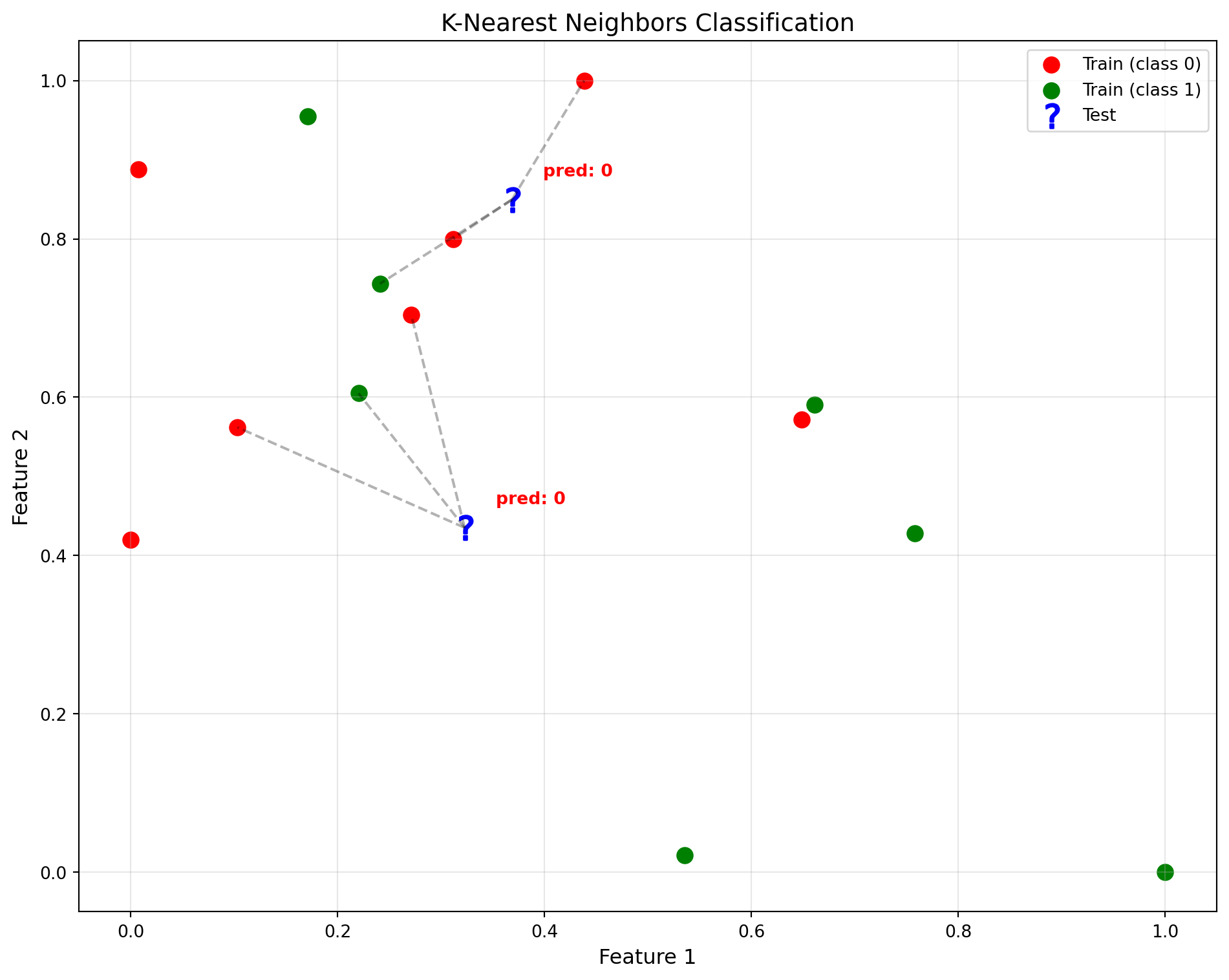

Unsupervised learning (TODO)

In this setting there is no known answer and the model tries to find structure in your data.

Example: video streaming service where your AI will group users by type based on infomration about content they have watched

Reinforcement learning

This is the type most people would think when thinking about AI. In this setting we’ll have “agents” that operate in an environment in a way that maximizes some kind of reward.

Example: software that controls your player character in a platform game. The reward is defined as the final score when passing a level. The agent is then trying to formulate rules for its behavior that maximize its score: this might include behavior that seeks to pick up score increasing power ups and avoiding hitting enemies and so on.