Inspired by metallurgy, simulated annealing is a technique used in mathematical optimization to find the best solution in complex problems.
Imagine climbing a mountain blindfolded. You’ll climb and as soon as you feel the next step is going down, you tell yourself that you reached the top. But that’s not always the case. Sometimes you’ll go down to reach another steap part of the mountain that will bring you higher. - That’s the greedy method
Another option is to start playing with probabilities. As said before, the next step could be acceptable even if you loose some altitude as long as there is a probability high enough (comapred to the altitude loss) that you’ll go up again. - That’s Simulated Annealing
Simulated Annealing
For this you’ll use the following formula: \(prob=exp(–(S_old–S_new)÷T)\)
where T is an bastract number (temperature) that you’ll decrease according to the amount of steps you’ll do to find a solution.
To start with code, here is what one iteration will look like:
import randomfrom math import expdef accept_prob(S_old, S_new, T):if S_new > S_old:return1.0else:return exp((S_new - S_old) / T)# the above function will be used as follows. this is shown just for# your information; you don't have to change anything heredef accept(S_old, S_new, T):if random.random() < accept_prob(S_old, S_new, T):print(True)else:print(False)accept(150,140,20)
True
Explanation
If the new state (S_new) is better than the old state (S_old), it is always accepted (probability = 1.0).
If S_new is worse than S_old, the function computes the probability of acceptance using the formula
If S_new is much worse than S_old, the exponent is negative and the probability is low.
If T is high, even bad moves have a higher chance of being accepted.
As T decreases, the probability of accepting worse solutions decreases, making the algorithm more selective over time.
Since the formula gives us a probability of 0.6065, This code will print True around 60% of the time
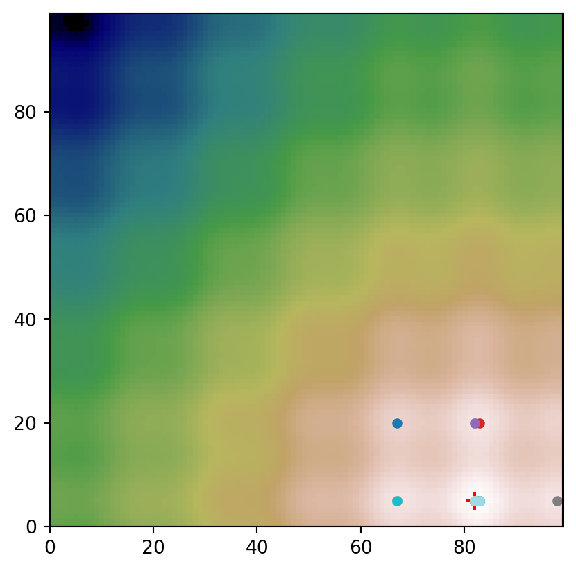
Ok so now let’s actually use this method in a mountain range and randomly place 50 people. This mountain range is a grid of 100 per 100 possible positions and we will resort to 3000 iterations to find the peak Our goal is for at least 30 to find the peak of the mountain range.
Note
We’ll also use a variation of geometric cooling to make sure the Temperature decreases gradually and starts at a certain value, gradually decreasing until reaching another certain value at the last iteration \(T = T_init * (T_final / T_init) ** (step / steps)\)
import numpy as npimport randomimport matplotlib.pyplot as pltfrom matplotlib import cmN =100# size of the problem is N x N steps =3000# total number of iterations tracks =50# generate a landscape with multiple local optima and set h with the value of the actual peak def generator(x, y, x0=0.0, y0=0.0):return np.sin((x/N-x0)*np.pi)+np.sin((y/N-y0)*np.pi)+\.07*np.cos(12*(x/N-x0)*np.pi)+.07*np.cos(12*(y/N-y0)*np.pi)x0 = np.random.random() -0.5y0 = np.random.random() -0.5h = np.fromfunction(np.vectorize(generator), (N, N), x0=x0, y0=y0, dtype=int)peak_x, peak_y = np.unravel_index(np.argmax(h), h.shape)# starting points x = np.random.randint(0, N, tracks)y = np.random.randint(0, N, tracks)# Min and max temperaturesT_init =20T_final =0.0001for step inrange(steps):# add a temperature schedule here T = T_init * (T_final / T_init) ** (step / steps)# update solutions on each search track for i inrange(tracks):# try a new solution near the current one x_new = np.random.randint(max(0, x[i]-2), min(N, x[i]+2+1)) y_new = np.random.randint(max(0, y[i]-2), min(N, y[i]+2+1)) S_old = h[x[i], y[i]] S_new = h[x_new, y_new]# if new solution is better or if there is a high probability of the next step being worth it, moveif S_new > S_old or random.random() < np.exp((S_new - S_old) / T): x[i], y[i] = x_new, y_new else:pass# if the new solution is worse, do nothing# Print results:print("Number of tracks found the peak:")print(sum([x[j] == peak_x and y[j] == peak_y for j inrange(tracks)])) # Print the actual plotplt.xlim(0, N-1)plt.ylim(0, N-1)plt.imshow(h, cmap=cm.gist_earth)plt.scatter([peak_y], [peak_x], color='red', marker='+', s=100)for j inrange(tracks): c = cm.tab20(j/tracks) # use different colors for different tracks plt.scatter([y[j]], [x[j]], color=c, s=20)plt.show()